
Some classic CNN
-->Please access the video via one of the following two ways
Some classic CNN models
In this section, we will use these convolutional operations introduced above to give a brief description of some classic convolutional neural network (CNN) models. Firstly, CNNS are actually a class of special DNN models. Let us recall the DNN structure as:
where
So the key features of CNNs is
Replace the general linear mapping to be convolution operations with multichannel.
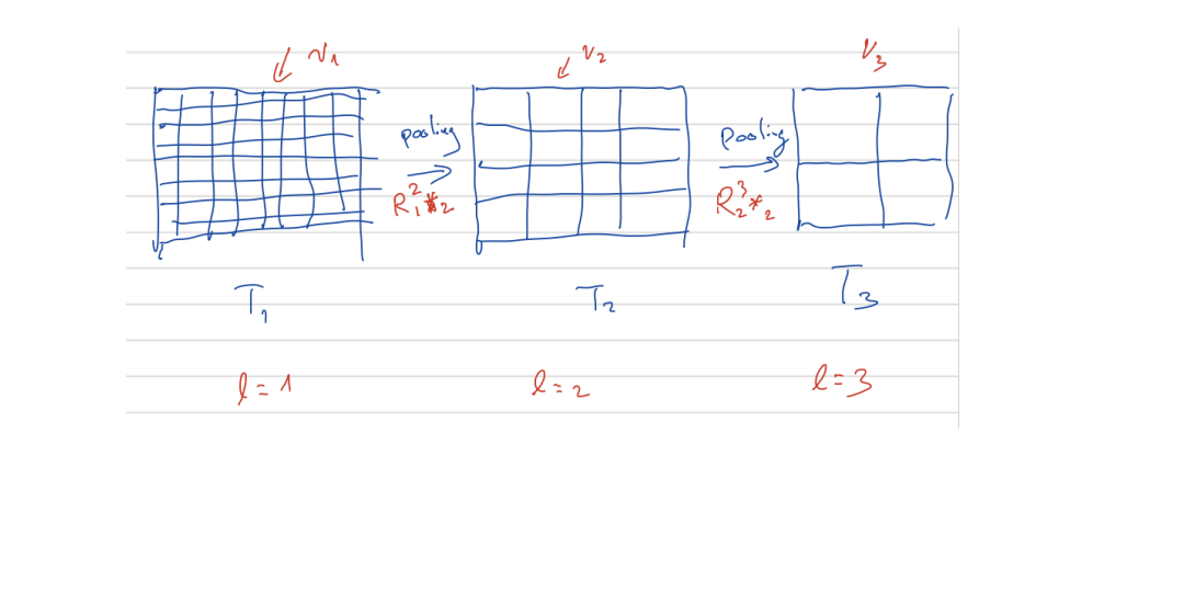
Use multi-resolution of images as shown in the next diagram.
Then we will introduce some classical architectures in convolution neural networks.
LeNet-5, AlexNet and VGG
The LeNet-5, AlexNet and VGG can be written as:
Algorithm 7 (\(h\) = Classic CNN\((f;J,v_1,\cdots,v_J)\))
Initialization \(f^{1,0} = f_{in}(f)\).
For \(l = i:J\) do
For \(i = 1:v_l\) do
Basic Block:
EndFor
Pooling(Restriction):
EndFor
Final average pooling layer: \(h = R_{ave}(f^{L,v_l})\)
Here \(R_{\ell}^{\ell+1} *_{2}\) represents for the pooling operation to sub-sampling these tensors into coarse spatial level (lower resolution). Here we use \(R_{\ell}^{\ell+1} *_{2}\) to stand for the pooling operation. In general we can also have
average pooling: fixed kernels such as
Max pooling \(R_{\max }\) as discussed before.
In these three classic CNN models, they still need some extra fully connected layers after \(h\) as the output of CNNs. After few layers of fully connected layers, the model is completed by following a multi-class logistic regression model.
These fully connected layers are removed in ResNet to be described below.
ResNet
The original ResNet is one of the most popular CNN architectures in image classification problems.
Algorithm 8 (\(h = ResNet(f;J,v_1,\cdots,v_J)\))
Initialization \(r^{1,0} = f_{in}(f)\)
For \(l = 1 : J\) do
For \(i=1:v_l\) do
Basic Block:
EndFor
Pooling(Restriction):
EndFor
Final average pooling layer: \(h=R_{ave }\left(r^{L, v_{t}}\right)\).
Here \(f_{\text {in }}(\cdot)\) may depend on different data set and problems such as \(f_{\text {in }}(f)=\sigma \circ \theta^{0} * f\) for CIFAR and \(f_{\text {in }}(f)=R_{\max } \circ \sigma \circ \theta^{0} * f\) for ImageNet [1] as in [3]. In addition \(r^{\ell, i}=r^{\ell, i-1}+A^{\ell, i} * \sigma \circ B^{\ell, i} * \sigma\left(r^{i-1}\right)\) is often called the basic ResNet block. Here, \(A^{\ell, i}\) with \(i \geq 0\) and \(B^{\ell, i}\) with \(i \geq 1\) are general \(3 \times 3\) convolutions with zero padding and stride 1. In pooling block, \(*_{2}\) means convolution with stride 2 and \(B^{\ell, 0}\) is taken as the \(3 \times 3\) kernel with same output channel dimension of \(R_{\ell}^{\ell+1}\) which is taken as \(1 \times 1\) kernel and called as projection operator. During two consecutive pooling blocks, index \(\ell\) means the fixed resolution or we \(\ell\)-th grid level as in multigrid methods. Finally, \(R_{\mathrm{ave}}\) \(\left(R_{\max }\right)\) means average (max) pooling with different strides which is also dependent on datasets and problems.
3 pre-act ResNet
The pre-act ResNet shares a similar structure with ResNet.
Algorithm 9 (\(h = pre-act ResNet(f;J,v_1,\cdots,v_J)\))
Initialization \(r^{1,0} = f_{in}f\)
For \(l = 1:J\) do
For \(i = 1:v_l\) do
Basic Block:
EndFor
Pooling(Restriction):
Here pre-act ResNet share almost the same setup with ResNet.
The only difference between ResNet and pre-act ResNet can be viewed as putting a \(\sigma\) in different places. The connection of those three models are often shown with next diagrams:
Without loss of generality, we extract the key feedforward steps on the same grid in different CNN models as follows.
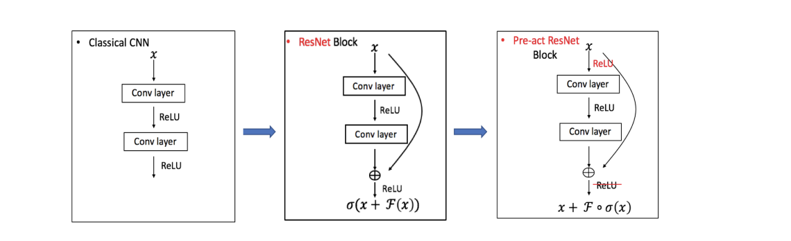
Fig. Comparison of CNN Structures
Classic CNN
ResNet
pre-act ResNet