Finite element method¶

-->

Please access the video via one of the following two ways

1. Google Drive: https://drive.google.com/drive/folders/1CfNBBbLwo-8V7JHfWQyd5-HCgRV0tRJ9?usp=share_link

2. Baidu Netdisk: https://pan.baidu.com/s/1yIrvhEHbiyNL5I3bgi6LTQ?pwd=tv61

Download the lecture notes here: Notes ¶

Finite element method is a classic numerical method for solving partial differential equations. In this chapter, we will give a brief introduction to this method. discuss its basic properties and error estimates. In later chapters, we will show that the neural network functions can be viewed as an extension of finite element function. In this chapter, we discuss the classical linear finite element spaces, the error estimate of the finite element method and adaptivity method to improve the approximation. For shape-regular mesh, we will establish both the upper and lower bound of the approximation error.

Linear finite element spaces¶

============================

In this section, we introduce linear finite element spaces. We will walk through the basic setup, and derive some error estimates.

Triangulations¶

Given a bounded polyhedral domain $\Omega \subset \mathbb {R}^d$, a geometric triangulation (also called mesh or grid) $\mathcal T_h=\{\tau\}$ of $ \Omega $ is a set of $d$-simplices such that

$\overline \Omega=\cup \tau$, where $ \overline \Omega$ denotes the closure of $\Omega$.
if $\tau_1$ and $\tau_2$ are distinct elements in $\mathcal T_h$ then $\stackrel{\circ}{\tau _1}\cap \stackrel{\circ}{\tau _2} = \varnothing$, where $\stackrel{\circ}{\tau _i}$ denotes the interior of $\tau_i, i=1,2$ .

Examples of triangulations for $\Omega=(0,1)$ ($d=1$) and for $\Omega=(0,1)^2$ ($d=2$) are shown in

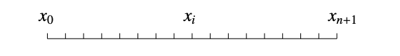
Fig. 6 1D uniform grid¶

and

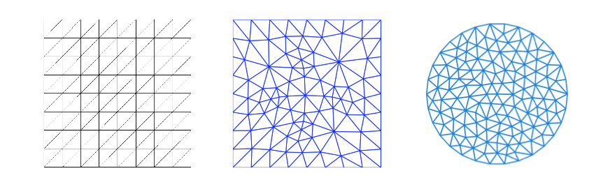
Fig. 7 2D uniform grid¶

Given $\Omega=(0,1)$, we consider the mesh:

(19)¶\[ 0=x_0<x_1<\cdots<x_{n+1}=1, \quad x_i=\frac{i}{n+1},\quad (i=0,\cdots,n+1) \]

which is the 1D uniform grid shown in figure Fig. 6

Denote

\[ h_\tau=\mbox{ diam} (\tau)\quad \hbox{(diameter of the smallest sphere containing $\overline{\tau}$)}, \]

and

\[ h=\max_{\tau\in\mathcal T_h} h_\tau;\quad \underline{h}=\min_{\tau\in\mathcal T_h} h_\tau. \]

A set of triangulations $\mathscr T$ is called shape regular if there exists a constant $c_0$ such that

(20)¶\[ \max _{\tau \in \mathcal T_h} \frac{h_{\tau}^d}{|\tau|}\leq c_0, \quad \forall \, \mathcal T_h\in \mathscr T \]

where $|\tau|$ is the measure of $\tau$ in $ R^d$. This assumption can also be represented as

(21)¶\[ \max_{\tau\in\mathcal T_h}\frac{h_\tau}{\rho_\tau}\le\sigma_1,\quad \forall \, \mathcal T_h\in \mathscr T \]

where $\rho_\tau$ denotes the radius of the ball inscribed in $\tau$. In two dimensions, it is equivalent to the minimal angle of each triange is bounded below uniformly in the shape regular class.

In addition to (20), if

(22)¶\[ \frac{\max _{\tau \in \mathcal T_h}|\tau|}{\min _{\tau \in \mathcal T_h}|\tau|} \leq \rho,\quad \forall \, \mathcal T_h\in \mathscr T \]

$\mathscr T$ is called quasi-uniform. For quasi-uniform grids, $h=\max _{\tau \in \mathcal T_h} h_{\tau}$, the mesh size of $\mathcal T_h$, is used to measure the approximation rate.

The assumption (22) is a local assumption, as is meant by above definition, for $d=2$ for example, it assures that each triangle will not degenerate into a segment in the limiting case. On the other hand, the assumption is a global assumption, which says that the smallest mesh size is not too small compared with the largest mesh size of the same triangulation. By the definition, in a quasi-uniform triangulation, all the elements are about the same size asymptotically.

Let $ x_{i}=(x^1_{i}, \cdots, x^d_{i})^t, i=1,\cdots, d+1$ be $d+1$ points in $ R^d$ which do not all lie in one hyper-plane. The convex hull of the $d+1$ points $ x_1, \cdots, x_{d+1}$ (See Figure [fig:barycentricCoor])

\[ \tau :=\{ x=\sum _{i=1}^{d+1}\lambda _i x_i \, | \, 0\leq \lambda_i\leq 1, i=1:d+1, \sum _{i=1}^{d+1}\lambda _i=1 \} \]

is defined as a geometric $d$-simplex generated (or spanned) by the vertices $ x_1, \cdots, x_{d+1}$. For example, a triangle is a $2$-simplex and a tetrahedron is a $3$-simplex. For an integer $0\leq m \leq d-1$, an $m$-dimensional face of $\tau$ is any $m$-simplex generated by $m+1$ of the vertices of $\tau$. Zero-dimenisonal faces are vertices and one-dimensional faces are called edges of $\tau$. The $(d-1)$-face opposite to the vertex $ x_i$ will be denoted by $F_i$.

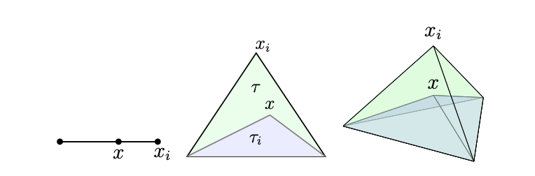
Fig. 8 Geometric explanation of barycentric coordinates¶

On the other hand, for any $ x\in \tau$, there exist unique numbers $\lambda _1,\cdots, \lambda _{d+1}$ satisfying $\displaystyle 0\leq \lambda_i\leq 1, i=1:d+1, \sum _{i=1}^{d+1}\lambda _i=1$ such that $\displaystyle x=\sum _{i=1}^{d+1}\lambda _i x_i$, thus we can denote $\lambda _1,\cdots, \lambda _{d+1}$ as $\lambda _1( x),\cdots, \lambda _{d+1}( x)$. In fact, the numbers $\lambda _1( x),\cdots, \lambda _{d+1}( x)$ are called barycentric coordinates of $ x$ with respect to the $d+1$ points $ x_1, \cdots, x_{d+1}$. There is a simple geometric meaning of the barycentric coordinates. Given a $ x\in \tau$, let $\tau _i( x)$ be the simplex with vertices $ x_i$ replaced by $ x$. Then it can be easily shown that

(23)¶\[ \lambda _i( x) = |\tau _i( x)|/|\tau|, \]

where $|\cdot|$ is the Lebesgure measure in $ R^d$, namely area in two dimensions and volume in three dimensions. Note that $\lambda _i( x)$ is affine function of $ x$ and vanishes on the face $F_i$. We list the four basic properties of barycentric coordinate below:

$0\leq \lambda_i( x)\leq 1$;
$\displaystyle\sum_{i=1}^{d+1} \lambda_i( x)=1$;
$\lambda_i( x)\in P_1(\tau)$, where $P_1(\tau)$ denotes the space of polynomials of degree $1$ (linear) on $\tau\in \mathcal T_h$;
$\lambda_i( x_j)=\delta_{ij}=\begin{cases} 1, \quad &\text{if} \quad i=j\\ 0, \quad &\text{if} \quad i\neq j \end{cases}.$

Continuous linear finite element spaces¶

A conforming linear finite element function in a domain $\Omega\subset \mathbb R^d$ is a continuous function that is piecewise linear function with respect to a grid or mesh consisting of a union of simplices.

Given a shape regular triangulation $\mathcal T_h$ of $\Omega$, we define the continuous linear finite element space as

(24)¶\[ V_h:=\{v\,|\, v\in C(\overline \Omega), \,\hbox{ and }\, v|_{\tau}\in P_1(\tau), \forall \tau \in \mathcal T_h\} \]

where $P_1(\tau)$ denotes the space of polynomials of degree $1$ (linear) on $\tau\in \mathcal T_h$. Whenever we need to deal with boundary conditions, we further define $V_{h,0}=V_h\cap H_0^1(\Omega)$.

We note here that the global continuity is also necessary in the definition of $V_h$ in the sense that if $u$ has a square interable gradient, that is $u\in H^1(\Omega)$, and $u$ is piecewise smooth, then $u$ is continuous.

We always use $n_h$ to denote the dimension of finite element spaces. For $V_h$, $n_h$ is the number of vertices of the triangulation $\mathcal T_h$ and for $V_{h,0}$, $n_h$ is the number of interior vertices.

Nodal basis functions and dual basis¶

For linear finite element spaces, we have the so called a standard nodal basis functions $\{\varphi _i,i=1,\cdots n_h\}$ such that $\varphi_i$ is piecewise linear (with respect to the triangulation) and $\varphi_i(x_j)=\delta_{i,j}$. Note that $\varphi _i|_\tau$ is the corresponding barycentrical coordinates of $x_i$. See Figure Fig. 10 for an illustration in 2D.

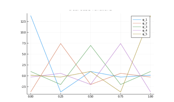
Fig. 9 Dual basis functions of Vh in 1D for nh = 5.¶

Let $(\varphi_i^*)_{i=1}^{n_h}$ be the dual basis of $(\varphi_i)_{i=1}^{n_h}$, namely

(25)¶\[ (\varphi_i^*, \varphi_j) =\delta_{i, j}, \quad i, j=1,\ldots, n_h \]

We notice that all the nodal basis functions $\{\varphi_i\}$ are locally supported, but their dual basis functions $\{\varphi_i^*\}$ are in general not locally supported (see Figure Fig. 9). The nodal basis functions $\{\varphi_i\}$ are easily constructed in terms of barycentric coordinate functions. The dual basis $\{\varphi_i^*\}$ are only interesting for theoretical consideration and it is not necessary to know the actual constructions of these functions.

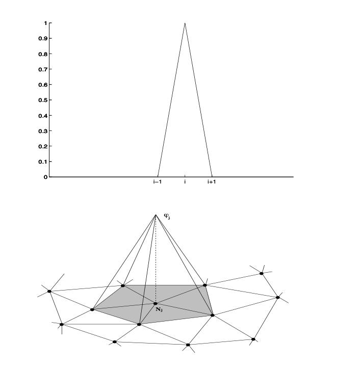
Fig. 10 Nodal basis functions in 1d and 2d¶

Since $\{\varphi_i,i=1,\cdots n_h\}$ is a basis of $V_h$, therefore for any $v_h\in V_h$, we have the representation

\[ v_h(x)=\sum_{i=1}^{n_h}v_h(x_i)\varphi_i(x) \]

Let us see how our construction of continuous linear finite space and the nodal basis looks like in one spatial dimension. Associated with the mesh

\[ \mathcal T_h=\{0=x_0<x_1<\ldots<x_{n_h}<x_{n_h+1}=1\} \]

by the definition given in (24) and the definition $V_{h,0}=V_{h}\cap H_0^1(\Omega)$, we have

\[ \begin{array}{ll} V_{h,0}=\{v:~\mbox{$v$ is continuous and piecewise linear}~ \mbox{w.~r.~t. $\mathcal T_h$, } v(0)=v(1)=0\}. \end{array} \]

A plot of a typical element of $V_{h,0}$ is shown in Figure Fig. 11

It is easily calculated (as we already mentioned), that the dimension of $V_{h,0}$ is equal to the number of internal vertices, and the nodal basis functions spanning $V_{h,0}$ (for $i=1,2,\cdots,n_h$) are (see also Fig Fig. 10

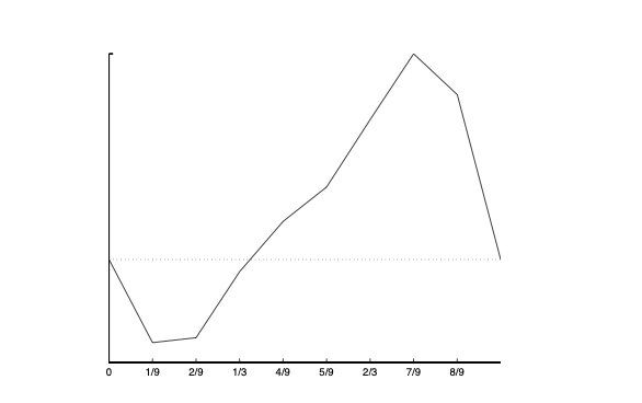
(26)¶\[\begin{split} \varphi_i(x)=\left\{\begin{array}{cl} \displaystyle \frac{x-x_{i-1}}{h}, & x\in[x_{i-1},x_i];\\ \displaystyle \frac{x_{i+1}-x}{h}, & x\in[x_{i},x_{i+1}];\\ 0 &\mbox{elsewhere}. \end{array}\right. \end{split}\]

Fig. 11 Plot of a typical element from Vh;0 .¶

Nodal value interpolant¶

For any continuous function $u$, we define its linear finite element interpolation, $(I_h u)(x)\in V_{h,0}$, as follows:

(27)¶\[ (I_h u)(x)= \sum_{i=1}^{n_h}u(x_i)\varphi_i(x) \]

Usually, we also denote $(I_h u)(x)$ as $u_I(x)$. Using interpolation, we can obtain the following approximation property of linear finite element space.

Theorem 5

Assume that $\mathcal T_h$ is quasi-uniform and $V_h$ is the linear finite element space associated with $\mathcal T_h$, then

(28)¶\[ \inf_{v_h\in V_h} \|v-v_h\|+h |v-v_h|_{1}\leq h^2 |v|_2 \forall v\in H^2(\Omega). \]

Proof. Proof Let us first prove Theorem Theorem 5 for $d=1, 2, 3$. Let $x=(x^1,\ldots, x^d)$ and $a_i=(a^1_{i}, \ldots, a^d_{i})$. Introducing the auxiliary functions

\[ g_i(t)=v(a_i(t)),\mbox{ with } a_i(t)=a_i+t(x-a_i) \]

we have

\[ g_i'(t)=(\nabla v)(a_i(t))\cdot (x-a_i) =\sum_{l=1}^d(\partial_lv)(a_i(t))(x^l-a_i^l) \]

and

(29)¶\[ g_i''(t)=\sum_{k,l=1}^d\partial^2_{kl}v)(a_i(t))(x^k-a_i^k)(x^l-a_i^l) \]

Note Taylor expansion

\[ g_i(0)=g_i(1)-g_i'(1)+\int_0^1tg''_i(t)dt \]

namely

(30)¶\[ v(a_i)=v(x)-(\nabla v)(x)\cdot (x-a_i)+\int_0^1tg''_i(t)dt \]

and note that

\[ (I_hv)(x)=\sum_{i=1}^{d+1}v(a_i)\lambda_i(x), \quad \sum_{i=1}^{d+1}\lambda_i(x)=1 \]

and

\[ \sum_{i=1}^{d+1}(x-a_i)\lambda_i(x)=0 \]

It follows that

(31)¶\[ (I_hv-v)(x)=\sum_{i=1}^{d+1}\lambda_i(x)\int_0^1tg''_i(t)dt \]

Using (29) and the trivial fact that $|x^l-a_i^l|\le h$, we obtain

\[ \begin{aligned} \|g''_i(t)\|_{L^2(\tau)}\le h^2 \sum_{k,l=1}^d\|(\partial^2_{kl}v)(a_i(t))\|_{L^2(\tau_i^t)} \le h^2t^{-d/2}\sum_{k,l=1}^d\|\partial^2_{kl}v\|_{L^2(\tau)},\end{aligned} \]

where we have used the following change of variable

\[ y=a_i+t(x-a_i): \tau\mapsto \tau_i^t\subset\tau \mbox{ with } dy=t^ddx \]

Now taking the $L^2(\tau)$ norm on both hand of sides of (31) , we get

\[\begin{split} \begin{aligned} \|I_hv-v\|_{L^2(\tau)} &\le& h^2\sum_{i=1}^{d+1}\max_{x\in\tau}|\lambda_i(x)| \int_0^1t\|g''_i(t)\|_{L^2(\tau)}\;dt\\ &\le& (d+1)\int_0^1t^{-d/2}dt\;h^2\; \sum_{k,l=1}^d\|\partial^2_{kl}v\|_{L^2(\tau)}\\ &\le&\frac{2(d+1)}{4-d}h^2 \sum_{k,l=1}^d\|\partial^2_{kl}v\|_{L^2(\tau)}\\ &\le&\frac{4d(d+1)}{4-d}h^2|v|_{H^2(\tau)}.\end{aligned} \end{split}\]

Now we prove the $H^1$ error estimate. Notice that

\[ [\partial_{j}( I_{h} v - v)](x) = \sum_{i} (\partial_{j} \lambda_{i} )(x) \int_{0}^{1} t g''_{i}(t) dt + \sum_{i} \lambda_{i}(x) \partial_{j} \int_{0}^{1} t g''_{i}(t) dt \]

By (30),

\[ \int_0^1tg''_i(t)dt = v(a_i) - v(x) + (\nabla v)(x)\cdot (x-a_i) \]

therefore,

\[\begin{split} \begin{aligned} \partial_{j} \int_0^1tg''_i(t)dt \\ & = & - \partial_{j} v + (\nabla \partial_{j} v )(x) (x - a_{i}) + \nabla v \cdot e_{j} \\ & = & (\nabla \partial_{j} v )(x) (x - a_{i}).\end{aligned} \end{split}\]

where $e_{j}$ is the $j$-th standard basis

Noting that $\sum_{i} \lambda_{i}( \nabla \partial_{j} v )(x) (x - a_{i}) = 0$, we have

\[ [\partial_{j}( I_{h} v - v)](x) = \sum_{i} (\partial_{j} \lambda_{i} )(x) \int_{0}^{1} t g''_{i}(t) dt \]

Then the estimate for $|\nabla(I_hv-v)|_{L^2(\tau)}$ follows by a similar argument and the following obvious estimate

\[ |(\nabla\lambda_i)(x)|\leq\frac{1}{h} \]

On the proof of Theorem Theorem 6 for $d\ge 4$, the above proof does not apply for $d \ge 4$. This is because when $d \ge 4$, the embedding relation between $H^{2}(\Omega) \hookrightarrow C(\bar{\Omega})$ is no longer true. Only continuous functions can have interpolations. In this case, one approach is to use the so-called Scott-Zhang interpolation

As a result of Theorem Theorem 5 , we have

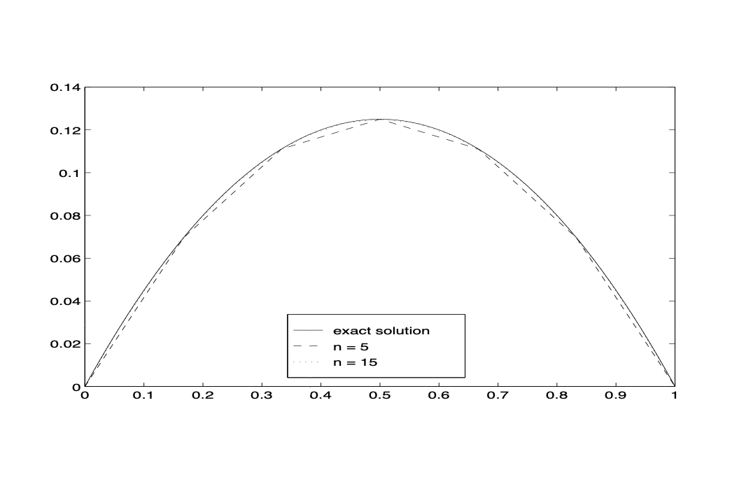
Fig. 12 Approximation of finite element space.¶

Theorem 6

Let $V_N$ be linear finite element space on a quasi-uniform triangulation consisting of $N$ element. Then

\[ \inf_{v_h\in V_N} \|v-v_h\|+N^{-{1\over d}} |v-v_h|_{1}\leq N^{-{2\over d}} |v|_2 \forall v\in H^2(\Omega) \]

Deep Learning Web Course

Finite element method¶

Please access the video via one of the following two ways

Download the lecture notes here: Notes¶

Linear finite element spaces¶

Triangulations¶

Continuous linear finite element spaces¶

Nodal basis functions and dual basis¶

Nodal value interpolant¶

Download the lecture notes here: Notes ¶