
Probabilistic derivation of logistic regression models
--> --> -->Please access the video via one of the following two ways
Probability interpretation of logistic regression
Logistic regression models the probabilities for classification problems with two possible outcomes. It’s an extension of the linear regression model for classification problems.
Input: d-dimension feature vector \(x\in R^{d}\)
Output: a class or label \(l \in\{1, \ldots, k\}\) (how to classify)
Example 1: Image classfication: Given input image \(x \in R^{n \times n}\), predict a label for the image. e.g. cat/ dog; MNIST: \(\{0, \ldots, 9\}\); CIFAR-10, \(\{0, \ldots, 9\}\)
Example 2: Binary Classfication: Given some medical data \(x\in R^{d}\)(features, like heart pressure, resting heart rate, family history, etc), we try to predict incidence of heart disease. The label will be binary \(\{0, 1\}\), called binary classification.
Logistic Regression Model
Given input feature vector \(x\in R^{n}\), the model predicts a probability distribution over the labels \(\{0, \ldots, k\}\).
with \(A\in R^{k \times n}\), \(x\in R^{n}\), \(b\in R^{k}\).
Softmax:
Input: \(y \in \mathbb{R}^{k}=\left(\begin{array}{l}y_{1} \\ \vdots \\ y_{k}\end{array}\right)\)
Output: Distribution \(p(j)=\frac{e^{y_{j}}}{\sum_{i=1}^{n} e^{y_{i}}}\)
Take exponential and normalize
Logistic Regression Model: Given input (feature/data) \(x \in R^{n}\), we return the distribution softmax \(\left( Ax+b\right)\) where A, b are parameters.
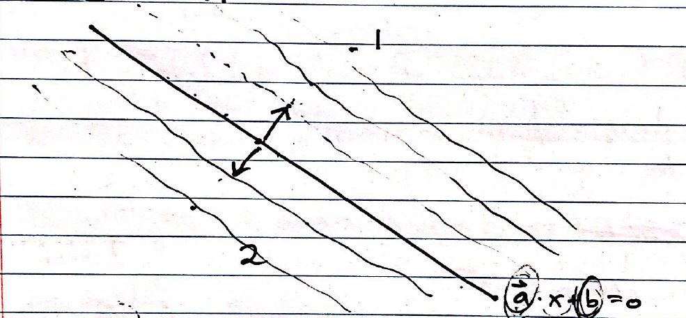
Example 1: Divide data into two classes: parameters are \(\vec{a}\in \mathbb{R}^{n}, b \in \mathbb{R}\)
\[ A\in \mathbb{R}^{1\times n},\quad Ax+b\in \mathbb{R}. \]The probability that the data \(x\) belongs to class 1 is
\[ P(1)=\frac{e^{\vec{a}\cdot x+b}}{e^{\vec{a} \cdot x+b}+1}, \]and the probability that the data \(x\) belongs to class 2 is
\[ P(2)=\frac{1}{e^{\vec{a} \cdot x+ b}+1}. \]If \(\vec{a} \cdot x+ b=0\), \(P(1)= P(2)={1\over 2}\). We don’t know how to classify the data lying on the line \(\vec{a} \cdot x+ b=0\) as shown in the figure below.
 {width=”.55\textwidth”}
Note that
By the above equation, \(\vec{a}\) means which feature is important. Logarithm of the odds: \(\log \left(\frac{p(1)}{p(2)}\right)\). Assumption: \(\log \left(\frac{p(1)}{p(2)}\right)\) is linear in the feature vector
Learning the parameters \(\vec{a}, b\) from data
Data: feature vectors \(x\) and corresponding labels \(l\). Given data
How can we estimate A, b?