Variational problems
Lemma 12
Assume that \(u\) is continuous in \((0,1)\), then the following
statements are equivalent
(1) \(u(x)=0\).
(2) \(\int_{0}^{1} u(x) v(x) d x=0\) for any smooth (compactly supported)
function \(v\) in \((0,1)\).
Define function \(v:[0,1] \rightarrow R\) and define space
\[
V=\{v: v \text { is continuous and } v(0)=v(1)=0\}
\]
Given any
\(f:[0,1] \rightarrow R\), consider
\[
J(v)=\frac{1}{2} \int_{0}^{1}\left|v^{\prime}\right|^{2} d x-\int_{0}^{1} f v d x
\]
Find \(u \in V\) such that
(38)\[
u=\underset{v \in V}{\arg \min } J(v)
\]
which
is equivalent to: Find \(u \in V\) such that
\[\begin{split}
\left\{\begin{array}{l}
-u^{\prime \prime}=f, 0<x<1, \\
u(0)=u(1)=0 .
\end{array}\right.
\end{split}\]
Proof. For any \(v \in V, t \in R\), let
\(g(t)=J(u+t v)\). Since \(u=\arg \min _{v \in V} J(v)\) means
\(g(t) \geq g(0) .\) Hence, for any \(v \in V, 0\) is the global minimum of
the function \(g(t)\). Therefore \(g^{\prime}(0)=0\) implies
\[
\int_{0}^{1} u^{\prime} v^{\prime} d x=\int_{0}^{1} f v d x \quad \forall v \in V
\]
By integration by parts, which is equivalent to
\[
\int_{0}^{1}\left(-u^{\prime \prime}-f\right) v d x=0 \quad \forall v \in V \text {. }
\]
By variational principal Lemma 12 , we obtain
\[\begin{split}
\left\{\begin{array}{l}
-u^{\prime \prime}=f, 0<x<1, \\
u(0)=u(1)=0 .
\end{array}\right.
\end{split}\]
Let \(V_{h}\) be finite element space and
\(\left\{\varphi_{1}, \varphi_{2}, \cdots \varphi_{n}\right\}\) be a nodal
basis of the \(V_{h} .\) Let
\(\left\{\psi_{1}, \psi_{2}, \cdots, \psi_{n}\right\}\) be a dual basis of
\(\left\{\varphi_{1}, \varphi_{2}, \cdots \varphi_{n}\right\}\), namely
\(\left(\varphi_{i}, \psi_{j}\right)=\delta_{i j} .\)
\[
J\left(v_{h}\right)=\frac{1}{2} \int_{0}^{1}\left|v_{h}^{\prime}\right|^{2} d x-\int_{0}^{1} f v_{h} d x .
\]
Let
\[
u_{h}=\sum_{i=1}^{n} v_{i} \varphi
\]
then
\[
u_{h}=\underset{v h \in V_{h}}{\arg \min } J\left(v_{h}\right)
\]
is equivalent to: Find \(u_{h} \in V_{h}\)
\[
a\left(u_{h}, v_{h}\right)=\left\langle f, v_{h}\right\rangle \quad \forall v_{h} \in V_{h}
\]
where
\[
a\left(u_{h}, v_{h}\right)=\int_{0}^{1} u_{h}^{\prime} v_{h}^{\prime} d x
\]
Which is equivalent to: Find \(u_{h} \in V_{h}\)
\[
a\left(u_{h}, v_{h}\right)=\left\langle f, v_{h}\right\rangle \quad \forall v_{h} \in V_{h}
\]
which is equivalent to solving \(\underline{A} \mu=b\), where
\(\underline{A}=\left(a_{i j}\right)_{i j}^{n}\) and
\(a_{i j}=a\left(\varphi_{j}, \varphi_{i}\right)\) and
\(b_{i}=\int_{0}^{1} f \varphi_{i} d x .\) Namely
\[\begin{split}
\frac{1}{h}\left(\begin{array}{ccccc}
2 & -1 & & & \\
-1 & 2 & -1 & & \\
& \ddots & \ddots & \ddots & \\
& & -1 & 2 & -1 \\
& & & -1 & 2
\end{array}\right)\left(\begin{array}{c}
\mu_{1} \\
\mu_{2} \\
\vdots \\
\mu_{n}
\end{array}\right)=\left(\begin{array}{c}
b_{1} \\
b_{2} \\
\vdots \\
b_{n}
\end{array}\right)
\end{split}\]
Which can be rewritten as
(39)\[
\frac{-\mu_{i-1}+2 \mu_{i}-\mu_{i+1}}{h}=b_{i}, \quad 1 \leq i \leq n, \quad \mu_{0}=\mu_{n+1}=0
\]
Using the convolution notation, (39) can be written as $\(A * \mu=b\)\(
where \)A=\frac{1}{h}[-1,2,-1]$
Introduction
Let us first briefly describe finite difference methods and finite
element methods for the numerical solution of the following boundary
value problem
(40)\[
-\Delta u=f, \text { in } \Omega, \quad u=0 \text { on } \partial \Omega, \quad Q=(0,1)^{2}
\]
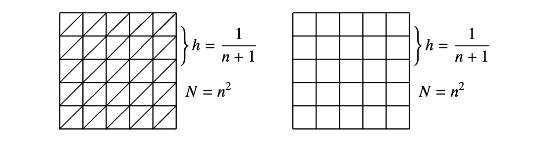
For the \(x\) direction and the \(y\) direction, we consider the partition:
\[\begin{split}
\begin{aligned}
&0=x_{0}<x_{1}<\cdots<x_{n+1}=1, \quad x_{i}=\frac{j}{n+1}, \quad(i=0, \cdots, n+1) \\
&0=y_{0}<y_{1}<\cdots<y_{n+1}=1, \quad y_{j}=\frac{j}{n+1}, \quad(j=0, \cdots, n+1)
\end{aligned}
\end{split}\]
Such a uniform partition in the \(x\) and \(y\) directions
leads us to a special example in two dimensions, a uniform square mesh
\(\mathbb{R}_{h}^{2}=\{(i h, j h) ; i, j \in \mathbb{Z}\}\).
Let \(\Omega_{h}=\Omega \cap \mathbb{R}_{h}^{2}\), the set of interior
mesh points and
\(\partial \Omega_{h}=\partial \Omega \cap \mathbb{R}_{h}^{2}\), the set
of boundary mesh points.\
Finite element methods
We consider two finite elements: continuous linear element and bilinear
element. These two finite element methods find \(u_{h} \in V_{h}\) such
that
\[
\left(\nabla u_{h}, \nabla v_{h}\right)=\left(f, v_{h}\right), \forall v_{h} \in V_{h}
\]
The above formulation can be written as
\[
\underline{A u}=\underline{f}
\]
with
\(\underline{A}_{(j-1) n+i,(l-1) n+k}=\left(\nabla \phi_{k l}, \nabla \phi_{i j}\right), f_{(j-1) n+i,(l-1) n+k}=\left(f, \phi_{i j}\right) .\)
Basis functions \(\phi_{i j}\) satisfy
\[
\phi_{i j}\left(x_{k}, y_{l}\right)=\delta_{(i, j),(k, l)}
\]
Linear finite element
Continuous linear finite element discretization of (40) on the left
triangulation in Fig 1.2. The discrete space for linear finite element
is
\[
\mathcal{V}_{h}=\left\{v_{h}:\left.v_{h}\right|_{K} \in P_{1}(K) \text { and } v_{h} \text { is globally continuous }\right\}
\]
Denote
\(E_{i, j}=\left[x_{i}, x_{i+1}\right] \times\left[y_{i}, y_{i+1}\right]=K_{i, j}^{U} \cup K_{i, j}^{D} .\)
For linear element case,
where
\[\begin{split}
A = \begin{pmatrix}
0 & -1 & 0\\
-1 & 4 & -1\\
0 & -1 & 0
\end{pmatrix}
\end{split}\]
and \(A * u \) is given by (41)
It is easy to verify that the formulation for the linear element method
is
(41)\[
4 u_{i, j}-\left(u_{i+1, j}+u_{i-1, j}+u_{i, j+1}+u_{i, j-1}\right)=f_{i, j}, \quad u_{i, j}=0
\]
if \(i\) or \(j \in\{0, n+1\}\)
where
\[
f_{i, j}=\int_{\Omega} f(x, y) \phi_{i, j}(x, y) \mathrm{d} x \mathrm{~d} y \approx h^{2} f\left(x_{i}, y_{j}\right)
\]
Proposition
The mapping A* has following properties
1- A is symmetric, namely
\[
(A * u, v)_{l^{2}}=(u, A * v)_{l^{2}} .
\]
2- \((A * v, v)_{F}>0\), if \(v \neq 0\).
3- \(A * u=f\) if and only if
\[
u \in \underset{v \in \mathcal{V}_{h}}{\arg \min } J(v)=\frac{1}{2}(A * v, v)-(f, v)
\]
4- The eigenvalues \(\lambda_{k l}\) and eigenvectors \(u^{k l}\) of A are
given by
\[\begin{split}
\begin{gathered}
\lambda_{k l}=4\left(\sin ^{2} \frac{k \pi}{2(n+1)}+\sin ^{2} \frac{l \pi}{2(n+1)}\right), \\
u_{i j}^{k l}=\sin \frac{k i \pi}{n+1} \sin \frac{l j \pi}{n+1}, 1 \leq i \leq n, 1 \leq j \leq n,
\end{gathered}
\end{split}\]
and \(\rho(A)<8 .\) Furthermore,
\[
\lambda_{n, n}=8 \cos ^{2} \frac{\pi}{2(n+1)} \approx 8\left(1-\left(\frac{\pi}{2(n+1)}\right)^{2}\right) \approx 8-\frac{2 \pi^{2}}{(n+1)^{2}}
\]
Bilinear element
Continuous bilinear finite element discretization of (40) on the right
mesh in Fig. 1.2. The discrete space for linear finite element is
\[
\mathcal{V}_{h}=\left\{v_{h}:\left.v_{h}\right|_{K} \in\{1, x, y, x y\} \text { and } v_{h} \text { is globally continuous }\right\}
\]
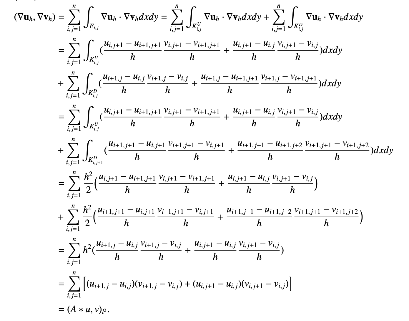
For bilinear element case, we have
\[\begin{split}
\begin{aligned}
\left(\nabla \mathbf{u}_{h}, \nabla \mathbf{v}_{h}\right)=& \sum_{i, j=1}^{n} \int_{E_{i, j}} \nabla \mathbf{u}_{h}, \nabla \mathbf{v}_{h} d x d y \\
=& \sum_{i, j=1}^{n} \int_{E_{i, j}}\left(\frac{\left(u_{i+1, j}-u_{i, j}\right)\left(y_{j+1}-y\right)}{h^{2}}+\frac{\left(u_{i, j+1}-u_{i+1, j+1}\right)\left(y-y_{j}\right)}{h^{2}}\right) \\
&\left(\frac{\left(v_{i+1, j}-v_{i, j}\right)\left(y_{j+1}-y\right)}{h^{2}}+\frac{\left(v_{i, j+1}-v_{i+1, j+1}\right)\left(y-y_{j}\right)}{h^{2}}\right) \\
&+\left(\frac{\left(u_{i, j+1}-u_{i, j}\right)\left(x_{i+1}-x\right)}{h^{2}}+\frac{\left(u_{i+1, j}-u_{i+1, j+1}\right)\left(x-x_{i}\right)}{h^{2}}\right) \\
=&\left(\frac{\left(v_{i, j+1}-v_{i, j}\right)\left(x_{i+1}-x\right)}{h^{2}}+\frac{\left(v_{i+1, j}-v_{i+1, j+1}\right)\left(x-x_{i}\right)}{h^{2}}\right) d x d y
\end{aligned}
\end{split}\]
where
\(A=\left(\begin{array}{ccc}-1 & -1 & -1 \\ -1 & 8 & -1 \\ -1 & -1 & -1\end{array}\right)\)
and \(A * u\) is given by (42)
And we have
(42)\[
8 u_{i j}-\left(u_{i+1, j}+u_{i-1, j}+u_{i, j+1}+u_{i, j-1}+u_{i+1, j+1}+u_{i-1, j-1}+u_{i-1, j+1}+u_{i+1, j-1}\right)=f_{i, j}
\]
and \(u_{i, j}=0\) if \(i\) or \(j \in\{0, n+1\} .\)